It is, expected
From Spot Price and Implied Volatility to Trading Reality


The art of trading options hinges on a deceptively simple yet profound principle: understanding where an underlying might move and how confident we should be in that projection. Two hours from now, a day from now, or weeks into the future—every trader wants to know the range of possibility. The answer lies in the marriage of two critical market inputs: today’s spot price and implied volatility. But the journey from these raw numbers to actionable expected move calculations reveals something unexpected about market efficiency and the surprising limits of our mathematical models.
At its core, answering the question “where will this underlying be in the future?” requires confronting the efficient market hypothesis head-on. The efficient market hypothesis presents a proposition that initially feels counterintuitive to anyone with strong market convictions: the best guess for any future price is simply the current price. Not higher, not lower—exactly where it is today, adjusted only marginally for the risk-free rate. This isn’t pessimism or resignation; it’s logical necessity. If the market’s collective participants believed the price would certainly be higher tomorrow, arbitrageurs would buy today, driving the price up immediately. Conversely, if everyone thought it would fall, they’d sell now, pushing it down. The market reaches equilibrium precisely at the point where no one can reliably guess the direction of the next move. Your bullish assumptions are irrelevant; the futures market—which sits at the pinnacle of price discovery—is always perfectly neutral on direction. You can argue for more or less volatility, but you cannot argue for directional bias without immediately confronting market resistance.
This principle, while sobering for directional traders, actually provides the foundation for understanding expected moves. The current price represents the centre of our distribution of future probabilities. The story doesn’t end there, however. That centre point is merely one dimension of the problem. What traders truly need to understand is the width of that distribution—how dispersed the possible outcomes are around that central price.
This is where implied volatility enters the picture as the critical variable. Imagine two identical underlyings: one trading at one hundred dollars with an implied volatility of fifteen percent, and another also trading at one hundred dollars with an implied volatility of fifty percent. Mathematically and intuitively, higher volatility should predict larger expected moves. The distribution around our central price remains centered at one hundred dollars in both cases, but one distribution is narrow and concentrated while the other is wide and dispersed. The same reasoning applies across time horizons. A one-month expected move will be smaller than a six-month expected move—but here’s where intuition begins to mislead us.
At first glance, one might assume that six times more days would produce six times more movement. After all, more calendar days means more price fluctuations, more ups and downs, more opportunity for significant changes. But when we account for the mathematics of how these movements compound over time, the scaling relationship proves more subtle. The market doesn’t move in a straight line; it moves in a random walk. Up moves and down moves partially cancel each other out. The further forward we project, the more opportunity there is for this cancellation to occur. Thus, the net expected change doesn’t scale linearly with time—it scales with the square root of time.
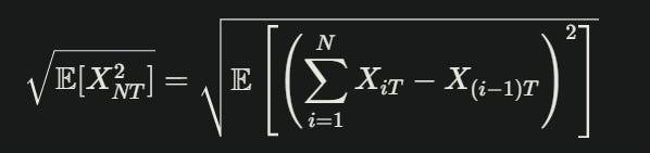
This mathematical relationship emerges from Brownian motion, the stochastic process that underpins modern financial theory. To understand why the square root of time governs this relationship requires diving into the mathematics, but the intuition is accessible. Imagine breaking a one-year period into twelve months. Each month generates its own expected move. These moves are independent—the direction of January’s movement tells us nothing about February’s direction. When we combine them into an annual expected move, we’re not simply adding them together. We’re adding their variances (the squares of the individual movements), then taking the square root of that sum. This is precisely where the square root of time emerges as the governing principle.
The mathematical machinery that produces this result depends on two critical assumptions: the efficient market hypothesis (which ensures that price movements in different time periods are independent of each other) and the linearity of expectations (which allows us to decompose complex distributions into simpler components). When we expand the variance formula and multiply out all the cross-terms where changes in one period interact with changes in another period, these cross-terms should theoretically vanish. Why? Because if the markets are efficient, those price changes are independent. Multiply two independent random variables with an expected value of zero together in expectation, and you get zero. The result is that only the sum of the squares of individual movements survives—and this leads directly to the square root scaling.
This visual shows the full derivation of the expected move formula for options pricing under the Efficient Market Hypothesis (EMH). The key steps are:
EMH Independence Property: The independence of returns over disjoint time intervals allows us to decompose the total duration into smaller intervals.
Initial Equation: